Understanding vector databases - Part 3
In this post, we will explore the tf-idf algorithm and observe how it facilitates the embedding of documents and words into vectors.
Here, we will focus on a collection of documents with the aim of comparing them and identifying those that exhibit similarities. As previously mentioned, our objective is to represent these documents as vectors. To achieve this, we will employ the tf-idf algorithm.
What is the tf-idf algorithm ?
The term frequency–inverse document frequency (tf-idf) algorithm is a numerical statistic that reflects the importance of a word in a document relative to a collection of documents, known as a corpus. It is commonly used in natural language processing and information retrieval to evaluate the significance of a term within a document.
The tf-idf algorithm relies on two key principles and common sense:
The more frequently a term appears in a specific document, the more likely it characterizes the content of that document. For instance, if the term "computer" is repeated 10 times in a particular document, it suggests that the document is likely to be about computers.
The more widespread a term is across all documents, the less discriminatory it is. For example, common English terms like "the" or "and" may appear in almost all documents, but they lack informative value about the specific focus of a document.
The first intuition is mathematically expressed through the term frequency (tf), while the second intuition is captured by the inverse document frequency (idf).
Compute the term frequence (tf)
This measures how frequently a term appears in a document. It is calculated as the number of occurrences of a term $t$ in a document $d$ divided by the total number of words in that document.
$$tf_{t,d}=log(1 + \dfrac{\text{number of times term } t \text{ appears in document }d}{\text{total number of terms in document }d})$$
Please note that there are various accepted formulas for calculating term frequency. Here, we are employing log normalization.
Compute the inverse document frequency (idf)
This quantifies how unique or rare a term $t$ is across all documents in the corpus. It is calculated as the logarithm of the total number of documents divided by the number of documents containing the term.
$$idf_{t}=log(\dfrac{\text{total number of documents in corpus}}{\text{number of documents containing term }t})$$
If a term $t$ is present in all documents, then $idf_{t}=0$.
Compute the tf-idf score
The tf-idf score for a term $t$ in a specific document $d$ is obtained by multiplying its term frequency (tf) by its inverse document frequency (idf).
$$\boxed{tfidf_{t, d}=tf_{t,d} * idf_{t}}$$
The resulting tf-idf scores provide a measure of the significance of each term within a document in relation to the entire corpus. Higher scores indicate terms that are important within a specific document but relatively rare across the entire collection.
If a term $t$ is present in all documents, then $idf_{t}=0$ and so $tfidf_{t, d}=0$. Hence, common words, often referred to as stop-words (in jargon), such as "the" or "and" will have a score of zero, signifying that they are non-discriminative and, therefore, not considered important. The advantage of tf-idf is that there is no need for preprocessing, such as eliminating these stop-words, before applying the algorithm.
Give me an example, please !
We will consider the following corpus (3 documents).
| document 1 | document 2 | document 3 |
|---|---|---|
| Microsoft Corporation, commonly known as Microsoft, is an American multinational technology company that produces, licenses, and sells computer software, consumer electronics, and other personal computing and communication products and services. Microsoft is one of the world's largest technology companies, founded by Bill Gates and Paul Allen in 1975. | Amazon.com, Inc. is an American multinational technology and e-commerce company based in Seattle, Washington. Founded by Jeff Bezos in 1994, Amazon started as an online bookstore and has since diversified into various product categories and services. It is one of the world's largest and most influential technology companies. | Renault is a French multinational automotive manufacturer established in 1899. The company produces a range of vehicles, from cars and vans to trucks and buses. Renault is known for its diverse lineup of vehicles and has a significant presence in the global automotive market. The company has been involved in various collaborations and partnerships with other automakers over the years. Additionally, Renault has a strong presence in motorsports and has achieved success in Formula One racing. |
There are 48 words in document 1, 49 words in document 2 and 76 words in document 3.
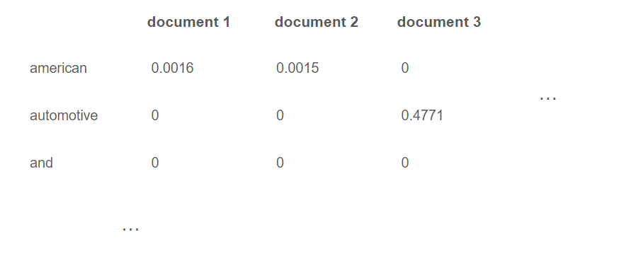
tf-idf for the term "american"
$tf_{american,1}=log(1+\dfrac{1}{48})=0.0089$ (american appears once), $tf_{american,2}=log(1+\dfrac{1}{49})=0.0088$ (american appears once) and $tf_{american,3}=log(1+\dfrac{0}{76})=0$ (american is not present).
$idf_{american}=log(\dfrac{3}{2})=0.1761$
Thus, $tfidf_{american,1}=(0.0089)(01761)=0.0016$, $tfidf_{american,2}=(0.0088)(01761)=0.0015$ and $tfidf_{american,3}=0$. The document 3 is inadequately represented by this term, aligning with both intuition and reality (Renault is a French company). Conversely, it aptly characterizes the other documents (Microsoft and Amazon are American companies).
tf-idf for the term "automotive "
$tf_{automotive ,1}=log(1+\dfrac{0}{48})=0$, $tf_{automotive ,2}=log(1+\dfrac{0}{49})=0$ and $tf_{automotive ,3}=log(1+\dfrac{2}{76})=0.0113$ (automotive appears twice).
$idf_{automotive}=log(\dfrac{3}{1})=0.4771$
Thus, $tfidf_{automotive,1}=0$, $tfidf_{automotive,2}=0$ and $tfidf_{automotive,3}=0.0113*0.4771=0.0054$. "automotive" stands out as a discriminative term, aligning once again with intuition.
tf-idf for the term "and"
The term "and" appears in all the documents, so $idf_{and}=0$ and thus $tfidf_{and,1}=tfidf_{and,2}=tfidf_{and,2}=0$. It reaffirms that there is no value in indicating the presence of the word "and" in each document.
What are the methods for leveraging the tf-idf algorithm for recommendations ?
Let $N$ represent the number of distinct terms in all the documents (in the corpus) and let's consider the vector space $\mathbb{R}^{N}$.
For each document, we will construct a vector in $\mathbb{R}^{N}$, where the $i$th component is the tf-idf score for the $i$th term in that document. As an illustration, let's examine how it works for our previous example with three documents.
Hence, the mathematical problem involves identifying, in an $N$-dimensional vector space, the 5 most similar (nearest) vectors to the current one. This requires introducing the concept of similarity, and, there are several ways to define this notion.
Jaccard similarity
The Jaccard similarity measures the similarity between two sets or two vectors. It is defined as the size of the intersection of the sets divided by the size of their union. In mathematical terms, if $A$ and $B$ are two sets, the Jaccard similarity $J(A,B)$ is $J(A,B)=\dfrac{\text{|}A\cap B\text{|}}{\text{|}A\cup B\text{|}}$.
The result is a value between 0 and 1, where 0 indicates no similarity (no common elements) and 1 indicates identical sets.
Cosine similarity
Cosine similarity is a measure of similarity between two non-zero vectors in an inner product space that measures the cosine of the angle between them.
Given two vectors $A$ and $B$, the cosine similarity $S(A,B)$ is calculated using the dot product of the vectors and their magnitudes.
$$S(A,B)=\dfrac{A.B}{\lVert A\rVert \rVert B\rVert}$$ Here, $A.B$ is the dot product of vectors $A$ and $B$, and $\rVert A\rVert$ and $\rVert B\rVert$ are the magnitudes (Euclidean norms) of vectors $A$ and $B$, respectively.
In our case, the cosine similarity ranges from 0 to 1, where 1 indicates that the vectors are pointing in the same direction, 0 indicates orthogonality (no similarity). In content-based recommendation, higher cosine similarity values between item feature vectors suggest greater similarity between items.
In the final post, we will briefly explore some algorithms utilized in vector databases to efficiently compute similarities.