Understanding time complexity on simple examples - Part 3
In this post, we will provide a concrete illustration of the concepts discussed by comparing various algorithms for calculating the power of a real number. We will demonstrate that certain methods are significantly more efficient than others.
Given a real number $x$ and an integer $n$, we aim to compute $x^n$ in an efficient manner. The code will be written in C#, but naturally, it is applicable to all other programming languages.
We will define an IComputePower interface that all algorithms will implement.
1public interface IComputePower
2{
3    double ComputePower(double real, int power);
4}
Algorithm 1
The first algorithm is quite straightforward and does not need further explanation: we are simply applying the mathematical definition of a power.
 1public class LinearComputePower : IComputePower
 2{
 3    public double ComputePower(double real, int power)
 4    {
 5        var y = 1.0;
 6        for (var i = 0; i < power; i++)
 7        {
 8            y *= real;
 9        }
10
11        return y;
12    }
13}
Analysis of the algorithm
We denote $T_{1}(n)$ as the number of multiplications performed during the execution of the program. It is evident from the code that $T_{1}(n)=n$ (as $n$ multiplications are performed in the for loop).
$$\boxed{T_{1}(n)=O(n)}$$
Algorithm 2
This second algorithm is merely a recursive variant of the first algorithm.
1public class LinearRecursiveComputePower : IComputePower
2{
3    public double ComputePower(double real, int power)
4    {
5        if (power == 0) return 1.0;
6        return real * ComputePower(real, power-1);
7    }
8}
Analysis of the algorithm
We denote $T_{2}(n)$ as the number of multiplications performed during the execution of the program. From the recursive form of the algorithm, we can express $T_{2}(n)=1+T_{2}(n−1)$ for all $n \ge 1$, with $T(0)=1$. This forms an induction relation that mirrors the recursive aspect of the code. The resolution of this induction is quite straightforward, and $T_{2}(n)=n$.
$$\boxed{T_{2}(n)=O(n)}$$
Algorithm 3
The third algorithm we are examining is a more intricate method, based on the fact that if $n$ is even, then $x^n=(x^2)^\dfrac{n}{2}$, and if $n$ is odd, then $x^n=x(x^2)^\dfrac{n-1}{2}$. This provides a dichotomic method that can be recursively implemented.
 1public class DichotomyComputePower : IComputePower
 2{
 3    public double ComputePower(double real, int power)
 4    {
 5        if (power == 0) return 1.0;
 6        if (power == 1) return real;
 7        else
 8        {
 9            if (power % 2 == 0) return ComputePower(real*real, power/2);
10            else return real * ComputePower(real*real, (power-1)/2);
11        }
12    }
13}
Analysis of the algorithm
We denote $T_{3}(x, n)$ as the number of multiplications performed during the execution of the program.
From the code, $T_{3}(x, n) = \begin{cases} 0 &\text{if } n=0 \text{ or } n=1 \\ 1+T_{3}(x^2, \lfloor\dfrac{n}{2}\rfloor) &\text{if } n \text{ is even} \\ 2+T_{3}(x^2, \lfloor\dfrac{n}{2}\rfloor) &\text{if } n \text{ is odd} \end{cases}$
$\lfloor\rfloor$ represents the integer part of a real number.
We can attempt to find an estimation of $T_{3}(x, n)$. Firstly, we express $n$ in base 2.
$$n=\displaystyle\sum_{i=0}^p a_{i}2^i$$
We have $a_{i}\in \lbrace0,1\rbrace$ for all $i \in \llbracket0,p-1\rrbracket$ and $a_{p}=1$.
If $p=0$, then $n=a_{0}$, and $T_{3}(x, n)=0$ according to the algorithm. Otherwise, when $p \ge 1$, $\dfrac{n}{2}=\dfrac{a_{0}}{2} + \displaystyle\sum_{i=0}^{p-1} a_{i+1}2^{i+1}$.
Thus, $\lfloor\dfrac{n}{2}\rfloor=\displaystyle\sum_{i=0}^{p-1} a_{i+1}2^{i+1}=\displaystyle\sum_{i=1}^{p} a_{i}2^{i}$.
If $a_{0}=0$, $n$ is even and $T_{3}(x, n)=1+T_{3}(x^2, \lfloor\dfrac{n}{2}\rfloor)$. If $a_{0}=1$, $n$ is odd and $T_{3}(x, n)=2+T_{3}(x^2, \lfloor\dfrac{n}{2}\rfloor)$.
Therefore, in all cases, $T_{3}(x, n)=1+a_{0}+T_{3}(x^2, \lfloor\dfrac{n}{2}\rfloor)$
By induction, we can conclude that $T_{3}(x, n)=\displaystyle\sum_{i=0}^{p-1} (1+a_{i})$
But $a_{i}\in \lbrace0,1\rbrace$ for all $i \in \llbracket0,p-1\rrbracket$ and $a_{p}=1$, so $p \le \displaystyle\sum_{i=0}^{p-1} (1+a_{i}) \le 2p$.
Additionally, as $n=\displaystyle\sum_{i=0}^p a_{i}2^i$, we have $2^p \le n \le 1+2+...+2^p = 2^{p+1}-1$, so $p \le log_{2}n$ on the one hand and $log_{2}(n+1)-1 \le p$ on the other hand.
Since $log_{2}(n+1)-1 \thicksim log_{2}n$, we eventually have $log_{2}n \le \displaystyle\sum_{i=0}^{p-1} (1+a_{i})=T_{3}(x, n) \le 2log_{2}n$
$$\boxed{T_{3}(x, n)=O(log_{2}n)}$$
This algorithm appears to have a very desirable execution time and is superior to the others.
How to verify our analyses ?
In this final section, we will attempt to demonstrate that our previous theoretical computations align with reality. To achieve this, we will intentionally introduce a Thread.Sleep instruction in our algorithm each time a multiplication is performed, and then we will execute the algorithms with various values of $n$.
For example, below is how our algorithm is modified with this instruction.
 1public class DichotomyComputePower : IComputePower
 2{
 3    public double ComputePower(double real, int power)
 4    {
 5        Thread.Sleep(1000);
 6
 7        if (power == 0) return 1.0;
 8        if (power == 1) return real;
 9        else
10        {
11            if (power % 2 == 0) return ComputePower(real*real, power/2);
12            else return real * ComputePower(real*real, (power-1)/2);
13        }
14    }
15}
The main program will utilize a watcher to calculate the execution time.
 1public static void Main(string[] args)
 2{
 3    var watch = new Stopwatch();
 4    var x = 2; var n = ...;
 5
 6    watch.Start();
 7
 8    var computer = new DichotomyComputePower();
 9    var res = computer.ComputePower(x, n);
10
11    watch.Stop();
12
13    Console.WriteLine($"Time elapsed: {watch.ElapsedMilliseconds} ms, result: {res}");
14}
Here are the results for various values of $n$.
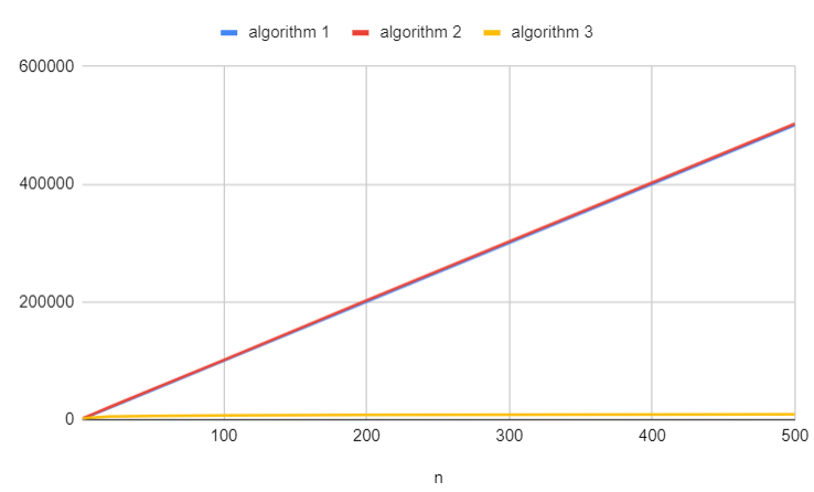
It is evident that the third algorithm executes faster than the others. This confirms our earlier analyses.
In the next article, we will continue our exploration with the study of linear recurrence sequences.