Neural networks for regression - a comprehensive overview - Part 3

In this post, we will briefly discuss how the backpropagation technique allows us to train a neural network for regression.

We will derive the different concepts using a 2-layer neural network. In this context, the neural network resembles the following diagram.

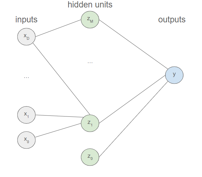
This scenario considerably simplifies the upcoming computations as there is only one output and two layers. We will by the way explicitly write down the mathematical relations involved, which would facilitate the upcoming explanations. We consider thus an input variable $X$ with $D$ features $x_{1}$, ..., $x_{D}$. We also introduce an extra input with activation fixed at $+1$ to not have to explicitely deal with the bias. $$a_{j}=\displaystyle\sum_{i=0}^Dw_{ji}x_{i}$$ $$z_{j}=\sigma (a_{j})$$ $$b=\displaystyle\sum_{j=0}^Mp_{j}z_{j}$$ $$y=b$$

Introducing the error function

We will assume that the training data (composed of $N$ elements $X_{1}$, ..., $X_{N}$ for inputs and $N$ elements $y_{1}$, ..., $y_{N}$ for outputs) is independent and identically distributed, implying that each data point is statistically independent of the others and originates from the same probability distribution. Each observation is presumed to be drawn independently from this common underlying probability distribution.
For regression problems, it is standard practice to use the sum-of-squares function to measure error, and we will adhere to this tradition.

$$\boxed{E(W)=\dfrac{1}{2}\displaystyle\sum_{i=1}^N(y_{i}-t_{i})^2}$$

Minimizing the cost function

Our goal is to find a vector $w$ such that $E(w)$ takes its smallest value.
Bishop (Pattern Recognition and Machine Learning)

What we aim to do now is minimize the cost function and the weights are the only things that we can vary to perform this task. Our goal is therefore to find $w_{00}$, ..., $w_{MD}$, $p_{0}$, ..., $p_{M}$ such that $E(W)$ is minimized. There are various methods for achieving this, such as different variants of gradient descent (stochastic gradient for example). We can also employ second-order derivative algorithms like the Newton-Raphson method or the L-BFGS algorithm.

In any case, we need to compute derivatives of the error function with respect to the parameters (this can be simply the gradient but also the Hessian). The difficulty with neural networks is that not all the quantities needed are directly accessible; for instance, for the output layer, we do not have access to the input layer, so we need to transition between the hidden layer to get them. This transition between layers relies, in mathematical terms, on the chain rule of differentiation. In fact, a quite efficient method has been proposed to compute these derivatives in the mid-80s and is referred to as backpropagation in the literature.

How to compute the gradient ?

The term backpropagation is often misunderstood as meaning the whole learning algorithm for multilayer neural networks. Actually, backpropagation refers only to the method for computing the gradient, while another algorithm (...) is used to perform learning using this gradient.
Goodfellow, Bengio, Courville (Deep Learning)

This citation is crucial to understand because we must emphasize that backpropagation only refers to an efficient method for computing derivatives, and these quantities can then be utilized with Newton or gradient-descent methods. We will dedicate this section to achieving this task in our regression scenario.

Note first that $E(W)=\displaystyle\sum_{n=1}^NE_{n}$ where $E_{n}=\dfrac{1}{2}(y_{n}-t_{n})^2$.

We will consider the problem of evaluating $\nabla E_{n}=(\dfrac{\partial E_{n}}{\partial w_{00}}, ..., \dfrac{\partial E_{n}}{\partial p_{M}})$ for one such term in the error function.

Computing $\dfrac{\partial E_{n}}{\partial p_{0}}$, ..., $\dfrac{\partial E_{n}}{\partial p_{M}}$

Let $j \in [0,M]$.

From the chain rule for partial derivatives, $\dfrac{\partial E_{n}}{\partial p_{j}}=\dfrac{\partial E_{n}}{\partial b_{n}}\dfrac{\partial b_{n}}{\partial p_{j}}$. This only involves the application of a well-known mathematical formula from calculus of variations.

As $b_{n}=\displaystyle\sum_{j=0}^Mp_{j}z_{j}$, it follows that $\dfrac{\partial b_{n}}{\partial p_{j}}=z_{j}$. Let $\delta_{n} = \dfrac{\partial E_{n}}{\partial b_{n}}$, the next step is to calculate $\delta_{n}$.

But $E_{n}=\dfrac{1}{2}(y_{n}-t_{n})^2$ and $y_{n}=b_{n}$, so $E_{n}=\dfrac{1}{2}(b_{n}-t_{n})^2$ and we eventually get the following formula.

$$\boxed{\delta_{n}=y_{n}-t_{n}}$$ $$\boxed{\dfrac{\partial E_{n}}{\partial p_{j}}=\delta_{n} z_{j}=(y_{n}-t_{n})z_{j}}$$

Computing $\dfrac{\partial E_{n}}{\partial w_{00}}$, ..., $\dfrac{\partial E_{n}}{\partial w_{MD}}$

Let $i \in [0,D]$ and $j \in [0,M]$.

From the chain rule for partial derivatives, $\dfrac{\partial E_{n}}{\partial w_{ji}}=\dfrac{\partial E_{n}}{\partial a_{j}}\dfrac{\partial a_{j}}{\partial w_{ji}}$.

As $a_{j}=\displaystyle\sum_{i=0}^Dw_{ji}x_{i}$, we have $\dfrac{\partial a_{j}}{\partial w_{ji}}=x_{i}$

Let $\delta_{nj}=\dfrac{\partial E_{n}}{\partial a_{j}}$.

$\delta_{nj}=\dfrac{\partial E_{n}}{\partial b_{n}}\dfrac{\partial b_{n}}{\partial a_{j}}$ (chain rule) and so $\delta_{nj}=\delta_{n} \dfrac{\partial b_{n}}{\partial a_{j}}$ where $\delta_{n}$ was defined above ($\delta_{n} = \dfrac{\partial E_{n}}{\partial b_{n}}$).

As $b_{n}=\displaystyle\sum_{j=0}^Mp_{j}z_{j}=\displaystyle\sum_{j=0}^Mp_{j}\sigma (a_{j})$, it follows that $\dfrac{\partial b_{n}}{\partial a_{j}}=p_{j}\sigma '(a_{j})$

$$\boxed{\delta_{nj}=\delta_{n} p_{j}\sigma '(a_{j})}$$ $$\boxed{\dfrac{\partial E_{n}}{\partial w_{ji}}=\delta_{nj}x_{i}=(y_{n}-t_{n})p_{j}\sigma '(a_{j})x_{i}}$$

Enter the backpropagation algorithm

The obtained mathematical formula furnishes us with the subsequent algorithm for assessing derivatives concerning the parameters.

• Initialize all parameters (weights) to small random values

• Repeat the following process for each input vector $X=(x_{1}, ..., x_{D})$ together with its target $t$.

  1. Forward propagate through the network to find the activations of all the hidden and output units $$a_{j}=\displaystyle\sum_{i=0}^Dw_{ji}x_{i}$$ $$z_{j}=\sigma (a_{j})$$ $$b=\displaystyle\sum_{j=0}^Mp_{j}z_{j}$$ $$y=b$$

  2. Evaluate $\delta$ for the output units $$\delta=y-t$$

  3. Backpropagate this error to obtain $\delta_{j}$ for each hidden unit $j$ $$\delta_{j}=\delta p_{j}\sigma '(a_{j})$$

  4. Evaluate the required derivatives with the following formula. $$\dfrac{\partial E_{n}}{\partial p_{j}}=\delta z_{j}$$ $$\dfrac{\partial E_{n}}{\partial w_{ji}}=\delta_{j}x_{i}$$

  5. Utilize these derivatives

We can, for instance, harness the stochastic gradient descent algorithm to effectuate an adjustment to the weight vector $W$. $$p_{j}^{new}=p_{j}^{old}-\eta \dfrac{\partial E_{n}}{\partial p_{j}}$$ $$w_{ji}^{new}=w_{ji}^{old}-\eta \dfrac{\partial E_{n}}{\partial w_{ji}}$$

The mathematical intricacies notwithstanding, in our upcoming post, we will transition to practical implementation by coding a neural network in C#.

Neural networks for regression - a comprehensive overview - Part 4