Neural networks for regression - a comprehensive overview - Part 2
In this post, we provide a brief overview of neural networks and discuss how to train them efficiently. We assume the reader has some prior knowledge of these data structures.
For those in need of a comprehensive introduction to neural networks, we recommend referring to the following article.
Implementing neural networks in C#
It provides an in-depth explanation of why these structures were developed, the problems they address, and how they can outperform some well-known algorithms.
What is a neural network ?
Neural networks were introduced to effectively capture non-linear relationships in data, where conventional algorithms like logistic regression struggle to model patterns accurately. While the concept of neural networks is not inherently difficult to grasp, practitioners initially faced challenges in training them (specifically, in finding the optimal parameters that minimize the loss function).
What problem are we trying to solve ?
The goal of machine learning is to predict an output based on given inputs. While this problem is not new, the vast amounts of data accumulated in recent years have allowed for more powerful and accurate predictions. Mathematically, the task involves using $D$ input features $x_{1}$, $x_{2}$, ..., $x_{D}$ to determine the $K$ corresponding outputs $y_{1}$, ..., $y_{K}$.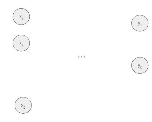
How do neural networks attempt to solve this problem ?
The most straightforward approach is to express the output directly as a function of the inputs.
$$(y_{1}, ..., y_{K})=f(x_{1}, ..., x_{D})$$
For example, a natural technique is to use a linear relationship between the inputs and the outputs.
$$y_{j}=\displaystyle\sum_{i=1}^D w_{ji}x_{i}$$
But what should we do when the relationship is clearly non-linear ? This is where neural networks come to the rescue. For a detailed explanation of how to progressively and intuitively arrive at the solution, we refer readers to the following article. Implementing neural networks in C#
- Construct $M$ linear combinations $a_{1}$, ..., $a_{M}$ of the input variables $x_{1}$, ..., $x_{D}$
$$a_{j}=\displaystyle\sum_{i=1}^D w_{ji}x_{i} + w_{j0}$$
What is $M$, and what does it stand for ? That is not very important for the moment, but the intuitive idea behind this formula is to construct a mapping from our original $D$-dimensional input space to another $M$-dimensional feature space. We will revisit this point later in this post.
- Each of these quantities is transformed using a differentiable, nonlinear activation function $h$.
$$z_{j}=h(a_{j})$$
- These values are again linearly combined to give $K$ output unit activations $b_{1}$, ..., $b_{k}$ (remember that $K$ is the count of classes).
$$b_{k}=\displaystyle\sum_{j=1}^M wo_{kj}z_{j} + wo_{k0}$$
- Finally, the output unit activations are transformed using an appropriate activation function to give a set of network outputs $y_{1}$, ,...,$y_{K}$.
$$y_{k}=\sigma (b_{k})$$
$\sigma$ can be the sigmoid (or other activation function) in the case of binary classification or the identity in the case of regression.
We can combine these various stages to give the overal network function.
$$y_{k}(x, w)=\sigma (\displaystyle\sum_{j=1}^M wo_{kj}h(\displaystyle\sum_{i=1}^D w_{ji}x_{i} + w_{j0}) + wo_{k0})$$
Thus the neural network model is simply a nonlinear function from a set of input variables $x_{1}$, ..., $x_{D}$ to a set of output variables $y_{1}$, ..., $y_{K}$ controlled by a vector $w$ of adjustable parameters.
Bishop (Pattern Recognition and Machine Learning)
We can observe that the final expression of the output is much more complex than that of simple logistic regression. This complexity provides flexibility, as now we will be able to model complex configurations (such as non-linearly separable data), but it comes at the expense of learning complexity. We now have many more weights to adjust, and the algorithms dedicated to this task are not trivial. It is this complexity that hindered neural network development in the late 80s.
The Universal Approximation Theorem is a foundational result in neural network theory that states a feedforward neural network with at least one hidden layer can approximate any continuous function, given certain conditions. This theorem highlights the power of neural networks in function approximation, regardless of the complexity or non-linearity of the function.
What is regression ?
Regression is a statistical and machine learning technique used to model and predict the relationship between a dependent variable (also known as the target or output) and one or more independent variables (known as features or inputs). The primary goal of regression is to understand how the dependent variable changes when one or more of the independent variables are modified, and to use this relationship to make predictions.
Regression is widely used for prediction tasks where the output is a continuous variable, making it an essential tool in both statistics and machine learning.
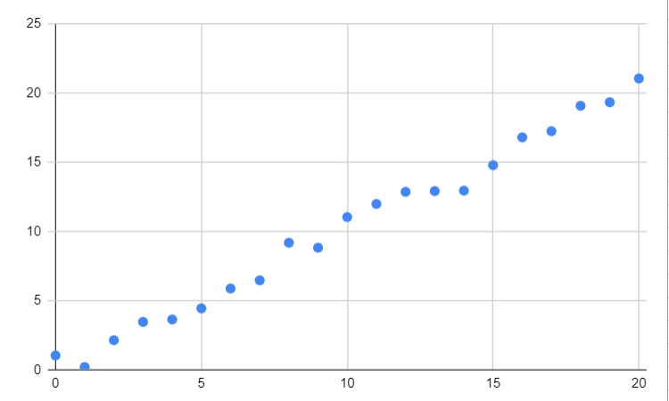
We've all encountered regression in school, often without realizing it. Anytime we used a formula to predict a value based on another variable (such as plotting a line through data points in a math or science class), we were practicing basic regression.
These examples from school are fairly simple because they typically involved just one input variable, and we applied linear regression, which was easy to visualize on a graph.
Applying linear regression in this context is quite straightforward (it's a common exercise often assigned to students as homework).
However, real-world scenarios are much more complex and often involve hundreds or even thousands of variables. In such cases, visual representation becomes impossible, making it much harder to assess whether our approximation is accurate.
Furthermore, deciding which type of regression to use becomes a critical question. Should we apply linear, quadratic, or polynomial regression ?
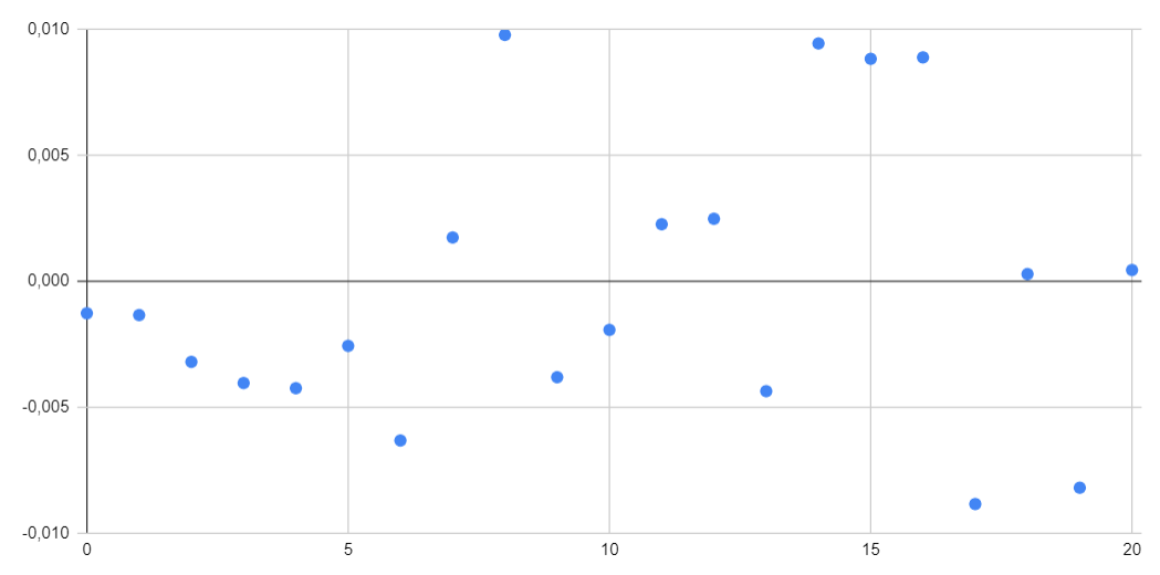
What type of regression should we use in this example ? Should we apply a sinusoidal regression or a polynomial one ? Even in this simple case, with only one input, it can be quite challenging to determine exactly which approach to choose.
Neural networks can come to the rescue by attempting to model the underlying function without the need to predefine the type of regression. This flexibility allows them to automatically capture complex patterns in the data, making it one of their greatest strengths. We will explore numerous examples throughout this series.
Integrating neural networks with regression
In the case of regression with neural networks, the output activation function is typically the identity function AND we will have only one output ($K=1$). This results in the following final formula, which we will use in the upcoming posts.
$$y(x, w)=\displaystyle\sum_{j=1}^M wo_{j}h(\displaystyle\sum_{i=1}^D w_{ji}x_{i} + w_{j0}) + wo_{0}$$
The formula may appear slightly simpler; however, the question of how to train the networks remains. Specifically, we need to determine how to find the optimal weights that minimize the loss function.
Neural networks for regression - a comprehensive overview - Part 3