Implementing neural networks in C# - Part 5
In this post, we will explore how to train the neural network and introduce the famous backpropagation algorithm for that purpose.
We will derive the different concepts within the context of binary classification (with classes $C_{1}$ and $C_{2}$) using a 2-layer neural network and refer to more specialized literature for regression and other scenarios. In this context, the neural network resembles the following diagram.
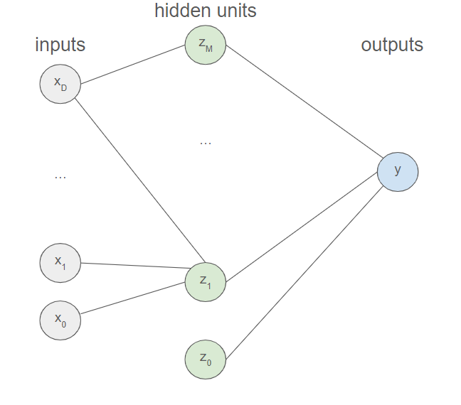
This scenario considerably simplifies the upcoming computations as there is only one output and two layers. We will by the way explicitly write down the mathematical relations involved, which would facilitate the upcoming explanations. We consider thus an input variable $X$ with $D$ features $x_{1}$, ..., $x_{D}$. We also introduce an extra input with activation fixed at $+1$ to not have to explicitely deal with the bias. $$a_{j}=\displaystyle\sum_{i=0}^Dw_{ji}x_{i}$$ $$z_{j}=\sigma (a_{j})$$ $$b=\displaystyle\sum_{j=0}^Mp_{j}z_{j}$$ $$y=\sigma(b)$$
Introducing the error function
We will assume that the training data (composed of $N$ elements $X_{1}$, ..., $X_{N}$) is independent and identically distributed, implying that each data point is statistically independent of the others and originates from the same probability distribution. Each observation is presumed to be drawn independently from this common underlying probability distribution. As a consequence, the joint probability is the product of the individual probabilities.
$$P(X_{1},...,X_{N})=P(X_{1})...P(X_{N})=\displaystyle\prod_{i=1}^NP(X_{i})$$
Let $i \in [1, N]$. If $X_{i}$ belongs to class $C_{1}$, then we have $P(X_{i})=P(C_{1}|X_{i})$. Otherwise, if $X_{i}$ belongs to class $C_{2}$, we have $P(X_{i})=P(C_{2}|X_{i})=1-P(C_{1}|X_{i})$. In all cases, we can express that $P(X_{i})=P(C_{1}|X_{i})^{t_{i}}(1-P(C_{1}|X_{i})^{1-t_{i}}$ where $t_{i}=1$ if $X_{i}$ belongs to class $C_{1}$ and $t_{i}=0$ if $X_{i}$ belongs to class $C_{2}$.
$$P(X_{1},...,X_{N})=\displaystyle\prod_{i=1}^NP(C_{1}|X_{i})^{t_{i}}(1-P(C_{1}|X_{i})^{1-t_{i}})$$
This quantity is commonly referred to as the likelihood.
The objective now is to maximize the likelihood. To avoid issues with underflows, it is common to work with the logarithm of this quantity. Since the logarithm function is monotonically increasing, it does not affect the optimization. The cost function $E(W)$ is then defined as the negation, and the goal is to minimize this quantity.
$$E(W)=-\ln{\displaystyle\prod_{i=1}^NP(C_{1}|X_{i})^{t_{i}}(1-P(C_{1}|X_{i})^{1-t_{i}})}$$
$$\boxed{E(W)=-\displaystyle\sum_{i=1}^N(t_{i}\ln{P(C_{1}|X_{i})}+(1-t_{i})\ln(1-P(C_{1}|X_{i})))}$$
This error function is commonly referred to as cross-entropy.
$W$ refers here to the $(M+)(D+1)$ weights $w_{00}$, ..., $w_{MD}$ of the first layer and the $M+1$ weights $p_{0}$, ..., $p_{M}$ of the second layer.
In our case, $P(C_{1}|X_{i})$ corresponds to the output of our neural network (it is indeed the result we aim to predict), so $P(C_{1}|X_{i})=y_{i}$.
$$\boxed{E(W)=-\displaystyle\sum_{i=1}^N(t_{i}\ln{y_{i}}+(1-t_{i})\ln(1-y_{i}))}$$
Minimizing the cost function
Our goal is to find a vector $w$ such that $E(w)$ takes its smallest value.
Bishop (Pattern Recognition and Machine Learning)
What we aim to do now is minimize the cost function and the weights are the only things that we can vary to perform this task. Our goal is therefore to find $w_{00}$, ..., $w_{MD}$, $p_{0}$, ..., $p_{M}$ such that $E(W)$ is minimized. There are various methods for achieving this, such as different variants of gradient descent (stochastic gradient for example). We can also employ second-order derivative algorithms like the Newton-Raphson method or the L-BFGS algorithm.
In any case, we need to compute derivatives of the error function with respect to the parameters (this can be simply the gradient but also the Hessian). The difficulty with neural networks is that not all the quantities needed are directly accessible; for instance, for the output layer, we do not have access to the input layer, so we need to transition between the hidden layer to get them. This transition between layers relies, in mathematical terms, on the chain rule of differentiation. In fact, a quite efficient method has been proposed to compute these derivatives in the mid-80s and is referred to as backpropagation in the literature.
How to compute the gradient ?
The term backpropagation is often misunderstood as meaning the whole learning algorithm for multilayer neural networks. Actually, backpropagation refers only to the method for computing the gradient, while another algorithm (...) is used to perform learning using this gradient.
Goodfellow, Bengio, Courville (Deep Learning)
This citation is crucial to understand because we must emphasize that backpropagation only refers to an efficient method for computing derivatives, and these quantities can then be utilized with Newton or gradient-descent methods. We will dedicate this section to achieving this task in our simple binary classification scenario.
Note first that $E(W)=\displaystyle\sum_{n=1}^NE_{n}$ where $E_{n}=-t_{n}\ln{y_{n}}-(1-t_{n})\ln(1-y_{n})$.
We will consider the problem of evaluating $\nabla E_{n}=(\dfrac{\partial E_{n}}{\partial w_{00}}, ..., \dfrac{\partial E_{n}}{\partial p_{M}})$ for one such term in the error function. This may be used directly for sequential optimization or the results can be accumulated over the training set in the case of batch methods.
Sequential and batch machine learning refer to different approaches in training machine learning models.
In sequential learning, the model is trained on one data point at a time. After processing each individual data point, the model's parameters (weights) are updated. This approach is well-suited for scenarios where new data becomes available continuously, and the model needs to adapt to changes over time (sequential learning is often used in real-time applications and online systems).
In batch learning, the model is trained on the entire dataset as a whole: the algorithm processes the entire dataset, computes the gradient of the cost function, and updates the model's parameters. This approach is suitable for scenarios where the entire dataset is available at once and can fit into memory (batch learning is often used in offline or batch processing scenarios, where the model is trained periodically on a fixed dataset).
For illustrative purposes, we will demonstrate sequential learning, although approaches involving batch learning are equally acceptable.
Computing $\dfrac{\partial E_{n}}{\partial p_{0}}$, ..., $\dfrac{\partial E_{n}}{\partial p_{M}}$
Let $j \in [0,M]$.
From the chain rule for partial derivatives, $\dfrac{\partial E_{n}}{\partial p_{j}}=\dfrac{\partial E_{n}}{\partial b_{n}}\dfrac{\partial b_{n}}{\partial p_{j}}$. This only involves the application of a well-known mathematical formula from calculus of variations.
As $b_{n}=\displaystyle\sum_{j=0}^Mp_{j}z_{j}$, it follows that $\dfrac{\partial b_{n}}{\partial p_{j}}=z_{j}$. Let $\delta_{n} = \dfrac{\partial E_{n}}{\partial b_{n}}$, the next step is to calculate $\delta_{n}$.
But $E_{n}=-t_{n}\ln{y_{n}}-(1-t_{n})\ln(1-y_{n})$ and $y_{n}=\sigma (b_{n})$, so we eventually get the following formula.
$$\delta=-t_{n}\dfrac{\sigma '(b_{n})}{\sigma (b_{n})}-(1-t_{n})(\dfrac{-\sigma '(b_{n})}{1-\sigma (b_{n})})$$
$$\boxed{\delta_{n}=y_{n}-t_{n}}$$ $$\boxed{\dfrac{\partial E_{n}}{\partial p_{j}}=\delta_{n} z_{j}=(y_{n}-t_{n})z_{j}}$$
Computing $\dfrac{\partial E_{n}}{\partial w_{00}}$, ..., $\dfrac{\partial E_{n}}{\partial w_{MD}}$
Let $i \in [0,D]$ and $j \in [0,M]$.
From the chain rule for partial derivatives, $\dfrac{\partial E_{n}}{\partial w_{ji}}=\dfrac{\partial E_{n}}{\partial a_{j}}\dfrac{\partial a_{j}}{\partial w_{ji}}$.
As $a_{j}=\displaystyle\sum_{i=0}^Dw_{ji}x_{i}$, we have $\dfrac{\partial a_{j}}{\partial w_{ji}}=x_{i}$
Let $\delta_{nj}=\dfrac{\partial E_{n}}{\partial a_{j}}$.
$\delta_{nj}=\dfrac{\partial E_{n}}{\partial b_{n}}\dfrac{\partial b_{n}}{\partial a_{j}}$ (chain rule) and so $\delta_{j}=\delta_{n} \dfrac{\partial b_{n}}{\partial a_{j}}$ where $\delta_{n}$ was defined above ($\delta_{n} = \dfrac{\partial E_{n}}{\partial b}$).
As $b_{n}=\displaystyle\sum_{j=0}^Mp_{j}z_{j}=\displaystyle\sum_{j=0}^Mp_{j}\sigma (a_{j})$, it follows that $\dfrac{\partial b_{n}}{\partial a_{j}}=p_{j}\sigma '(a_{j})$
$$\boxed{\delta_{nj}=\delta_{n} p_{j}\sigma '(a_{j})}$$ $$\boxed{\dfrac{\partial E_{n}}{\partial w_{ji}}=\delta_{nj}x_{i}=(y_{n}-t_{n})p_{j}\sigma '(a_{j})x_{i}}$$
Enter the backpropagation algorithm
The obtained mathematical formula furnishes us with the subsequent algorithm for assessing derivatives concerning the parameters.
Initialize all parameters (weights) to small random values
Repeat the following process for each input vector $X=(x_{1}, ..., x_{D})$ together with its target $t$ ($t=0$ or $t=1$).
Forward propagate through the network to find the activations of all the hidden and output units $$a_{j}=\displaystyle\sum_{i=0}^Dw_{ji}x_{i}$$ $$z_{j}=\sigma (a_{j})$$ $$b=\displaystyle\sum_{j=0}^Mp_{j}z_{j}$$ $$y=\sigma(b)$$
Evaluate $\delta$ for the output units $$\delta=y-t$$
Backpropagate this error to obtain $\delta_{j}$ for each hidden unit $j$ $$\delta_{j}=\delta p_{j}\sigma '(a_{j})$$
Evaluate the required derivatives with the following formula. $$\dfrac{\partial E_{n}}{\partial p_{j}}=\delta z_{j}$$ $$\dfrac{\partial E_{n}}{\partial w_{ji}}=\delta_{j}x_{i}$$
Utilize these derivatives
We can, for instance, harness the stochastic gradient descent algorithm to effectuate an adjustment to the weight vector $W$. $$p_{j}^{new}=p_{j}^{old}-\eta \dfrac{\partial E_{n}}{\partial p_{j}}$$ $$w_{ji}^{new}=w_{ji}^{old}-\eta \dfrac{\partial E_{n}}{\partial w_{ji}}$$
The backpropagation method elucidated herein has been formulated for the straightforward scenario of binary classification involving a single output and merely two layers. The broader context, encompassing multiple outputs and an unspecified number of layers, introduces added complexity; nevertheless, the underlying philosophy persists unchanged.
The mathematical intricacies notwithstanding, in our upcoming post, we will transition to practical implementation by coding a neural network in C#.