Implementing decision trees with the C4.5 algorithm - Part 4
In this final article, we explore the C4.5 algorithm as an enhancement of the ID3 algorithm and how to implement it in ML.NET.
What id the C4.5 algorithm ?
The C4.5 algorithm is a successor to the ID3 algorithm. C4.5 was developed by Ross Quinlan with improvements in handling both categorical and continuous data, as well as handling missing values. While ID3 works well with categorical data, C4.5 introduces a mechanism to handle continuous data by selecting optimal thresholds for splitting. This allows C4.5 to be more versatile in handling different types of datasets.
In summary, the C4.5 algorithm is an extension and improvement upon the ID3 algorithm, making it more robust and applicable to a broader range of datasets, including those with continuous attributes and missing values.
Additionally, C4.5 incorporates a pruning mechanism to avoid overfitting. After building the tree, it may be pruned by removing branches that do not significantly improve the model's accuracy on unseen data. This helps prevent the tree from becoming too complex and specific to the training data, promoting better generalization. ** We won't cover this aspect in this post.**
Understanding drawbacks of the information gain
The ID3 algorithm is straightforward to comprehend and implement, especially once we grasp the concept of entropy. However, this simplicity conceals several significant drawbacks. For instance, in the dataset we previously utilized, the distribution of different values for a specific feature was well spread out.
| Height | Hair | Eyes | Attractive ? |
|---|---|---|---|
| Small | Blonde | Brown | No |
| Tall | Dark | Brown | No |
| Tall | Blonde | Blue | Yes |
| Tall | Dark | Blue | No |
| Small | Dark | Blue | No |
| Tall | Red | Blue | Yes |
| Tall | Blonde | Brown | No |
| Small | Blonde | Blue | Yes |
Indeed, the dataset comprises a total of 8 rows. Among these 8 rows, the Height feature has two different values quite evenly distributed (3 Small and 5 Tall), the Hair feature has three different values quite evenly distributed (4 Blonde, 3 Dark and 1 Red), and the Eyes feature has two different values quite evenly distributed (3 Brown and 5 Blue).
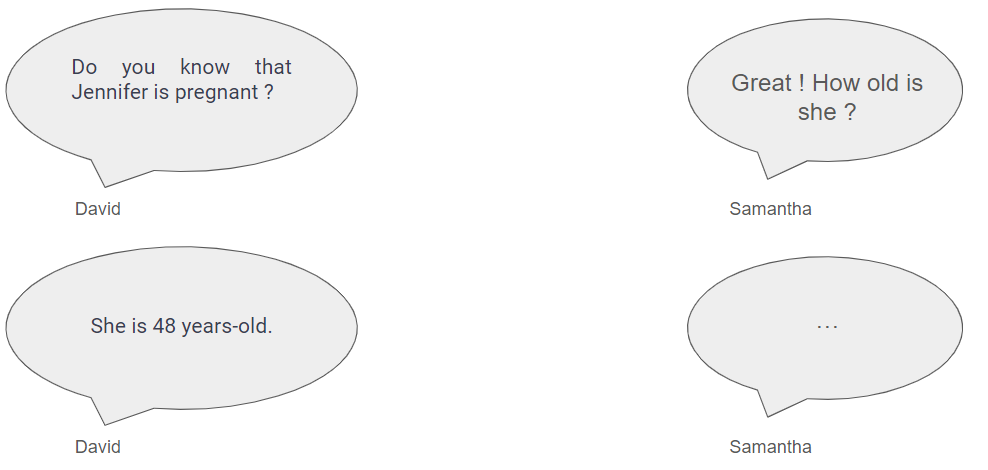
But consider now a dataset where one of the features is the age of a woman's first pregnancy. Typically, in many countries, women have their first children between 20 and 35 years old. However, there may be cases where some women have children after 40 and even up to 50, but these instances are relatively rare.
The dataset could anyway ressemble the following.
| Age first pregnancy | Hair | Working status |
|---|---|---|
| 15 | Blonde | Unemployed |
| 15 | Dark | Unemployed |
| ... | ... | ... |
| 25 | Blonde | Employed |
| 25 | Dark | Employed |
| ... | ... | ... |
| 28 | Dark | Unemployed |
| 28 | Dark | Employed |
| ... | ... | ... |
| 35 | Dark | Unemployed |
| 35 | Blonde | Employed |
| ... | ... | ... |
| 42 | Dark | Unemployed |
| 44 | Dark | Employed |
| 48 | Blonde | Employed |
| 50 | Blonde | Unemployed |
This dataset could comprise a total of 10000 rows. Among these 10000 rows, the Age first pregnancy feature has 36 different values that are extremely poorly distributed (800 25, 850 28, 1 44, 0 46, 1 50 for instance). This poor distribution will lead to high entropy (uncertainty is low), resulting in high information gain. Consequently, this feature will be chosen to split the data. But how will the tree be constructed then ?
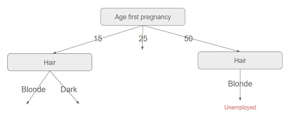
The tree will be able to split the data further for women whose age at first pregnancy is 25, 28, or 35. But how can it proceed for the woman whose age at first pregnancy is 50 ? As there is only one example, it will simply copy the data of this example (with Hair=Blonde). Now, what will happen if a dark-haired 50-year-old woman is tested against this decision tree ? As there is no path with these attributes, it will return the only value it can. In fact, here, this portion of the tree is too tailored to the training dataset.
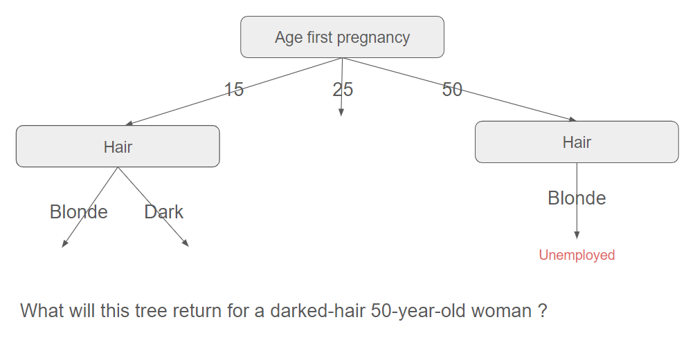
This illustrates overfitting: the dataset fits the training example very well but does not generalize well to other sets.
Information gain is biased toward high branching features.
Entering gain ratio
To mitigate the bias introduced by information gain, another heuristic was proposed by Quinlan and named gain ratio ($IGR$). He first defines the split information value for a specific feature $f$ as follows.
$$SplitInformation(S,f)=-\displaystyle\sum_{i=1}^{N} \dfrac{N(x_{i})}{N(S)} log_{2}\dfrac{N(x_{i})}{N(S)}$$
$x_{1}$, $x_{2}$, ..., $x_{N}$ are the different possible values for $f$ and $N(x_{i})$ are the number of times that $x_{i}$ occurs divided by the total count of events $N(S)$ for all $i \in [1,N]$.
Then, he defines the gain ratio $IGR(S,f)$ for this feature as simply the ratio of the information gain $IG(S,f)$ and the split information.
$$IGR(S,f)=\dfrac{IG(S,f)}{SplitInformation(S,f)}$$
The intuition behind this formula is that low entropy caused by features with a high number of distinct values (like our example above), results in a higher split information. Therefore, the information gain ratio is lower.
A worked example, please !
We will revisit the example from the previous post regarding which features are important for the attractiveness of a person. Below, we have copied the information gains that we had calculated earlier.
$$IG(S,Height)=0.004$$ $$IG(S,Hair)=0.454$$ $$IG(S,Eyes)=0.348$$
From the above formula, we have for example $SplitInformation(S,Height)=-\dfrac{3}{8}log_{2}\dfrac{3}{8}-\dfrac{5}{8}log_{2}\dfrac{5}{8}=0.954$ (5 records labeled as "Tall" and 3 labeled as "Small").
$$IGR(S,Height)=\dfrac{IG(S,Height)}{SplitInformation(S,Height)}=0.004$$
The reader is invited to perform the remaining calculations, and we'll proceed to present the results below.
| IG | SplitInformation | IGR | |
|---|---|---|---|
| Height | 0.004 | 0.954 | 0.004 |
| Hair | 0.454 | 1.406 | 0.323 |
| Eyes | 0.348 | 0.954 | 0.365 |
In this example, we can observe that the gain ratio has favored the feature with the fewer number of distinct values (Eyes, which can take only Brown and Blue) and penalized the Hair feature. Consequently, the data is now split with the Eyes feature first, in contrast to the Hair feature as discussed in the previous post.
The C4.5 algorithm (using the gain ratio) is less prone to overfitting compared to its ID3 counterpart.
How to deal with continuous features ?
Another limitation of the ID3 algorithm is the challenge it faces when dealing with continuous variables. The C4.5 algorithm attempts to address this issue and we will modify our example by replacing the Height feature with numerical values to see it in action.
| Height (cm) | Hair | Eyes | Attractive ? |
|---|---|---|---|
| 160 | Blonde | Brown | No |
| 186 | Dark | Brown | No |
| 188 | Blonde | Blue | Yes |
| 184 | Dark | Blue | No |
| 162 | Dark | Blue | No |
| 192 | Red | Blue | Yes |
| 188 | Blonde | Brown | No |
| 160 | Blonde | Blue | Yes |
The C4.5 algorithm proposes to perform binary split based on a threshold value. This threshold should be a value which offers maximum gain for that attribute.
- Sort the different values for Height in the ascending order: 160, 162, ..., 192.
- For each value $h$, partition the records into two groups: one with Height values up to and including $h$ and the other with values greater than $h$.
- For each of these partitions, compute the gain ratio.
- Choose the partition that maximizes the gain
A worked example again !
Remember that for our toy example, $H(S)=0.954$
Sort the different values for Height in the ascending order. There are 6 distinct values for the Height feature: 160, 162, 184, 186, 188, 192.
For each value $h$, partition the records into two groups: one with Height values up to and including $h$ (dataset named $H_{Height\le h}$) and the other with values greater than $h$ (dataset named $H_{Height\gt h}$).
For $h=160$ for instance, $H_{Height\le 160}$ comprises 2 records.
| Height (cm) | Hair | Eyes | Attractive ? |
|---|---|---|---|
| 160 | Blonde | Brown | No |
| 160 | Blonde | Blue | Yes |
$H_{Height\gt 160}$ comprises 6 records.
| Height (cm) | Hair | Eyes | Attractive ? |
|---|---|---|---|
| 162 | Dark | Blue | No |
| 184 | Dark | Blue | No |
| 186 | Dark | Brown | No |
| 188 | Blonde | Blue | Yes |
| 188 | Blonde | Brown | No |
| 192 | Red | Blue | Yes |
- Compute the gain ratio
We have $H(H_{Height\le 160})=1$ and $H(H_{Height\gt 160})=-\dfrac{4}{6}log_{2}\dfrac{4}{6}-\dfrac{2}{6}log_{2}\dfrac{2}{6}=0.918$.
It follows that $IG(S,Height_{160})=H(S)-(\dfrac{2}{8}H(H_{Height\le 160})+\dfrac{6}{8}H(H_{Height\gt 160}))=0.016$
Since $SplitInformation(S,Height_{160})=-\dfrac{2}{8}log_{2}\dfrac{2}{8}-\dfrac{6}{8}log_{2}\dfrac{6}{8}=0.811$, we eventually get $IGR(S,Height_{160})=0.020$
- Repeat this operation for all the distinct values
| $h$ (cm) | $IG(S,Height_{h})$ | $SplitInformation(S,Height_{h})$ | $IGR(S,Height_{h})$ |
|---|---|---|---|
| 160 | 0.016 | 0.811 | 0.020 |
| 162 | 0.003 | 0.954 | 0.003 |
| 184 | 0.049 | 1.000 | 0.049 |
| 186 | 0.159 | 0.954 | 0.167 |
| 188 | 0.074 | 0.544 | 0.136 |
- Choose the partition that maximizes the gain
Thus, if we were to split the data using the Height feature, we would need to set the threshold at 186 cm.
This method involves a substantial number of computations.
It's a bit of theory! We will now put this into practice and see how to leverage ML.NET to witness decision trees in action. This will be the subject of the next article.