Implementing decision trees with the C4.5 algorithm - Part 3
In this article, we delve into the intricacies of the ID3 algorithm, applying the knowledge we've acquired to gain a profound understanding of its workings.
Decision trees possess a simplicity that renders them accessible to both novices and seasoned machine learning practitioners. Operating akin to a rules-based engine, their decision-making process is easily explicable, making them a pivotal data structure in the realm of machine learning.
The current challenge lies in automating the construction of these decision trees, and our journey begins by delving into the ID3 algorithm.
The goal is indeed to construct the tree, but the real challenge lies in obtaining the smallest possible tree to ensure quick usage when classifying an unknown input.
What is the ID3 algorithm ?
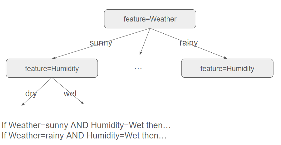
We must be aware that several trees can be built based on the features we successively consider. For instance, with the example above, we could start with the Humidity feature instead of the Weather feature.
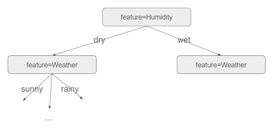
As there are various ways to construct the tree, we thus need to rely on heuristics to build it. And the heuristic is as follows: the algorithm constructs the tree in a greedy manner, starting at the root and selecting the most informative feature at each step.
This last sentence contains two important intuitions.
- Construct in a greedy manner: It appears intuitive and natural to split based on the feature that provides the most information.
- Select the most informative feature: The concept of the most informative feature might seem informal initially, but fortunately, we learned in the previous article how to define this concept mathematically. Therefore, we will choose the feature with the highest entropy, indicating the highest quantity of information.
OK, but it is lots of theory. Can you give me an example, please ?
Instead of using the conventional example about playing golf or not, we will leverage the following (politically incorrect) data to see ID3 in action. In this dataset, three features (Height, Hair, and Eyes) are provided along with a target variable (Attractive). The objective is to classify which attributes contribute to a person being considered attractive.
| Height | Hair | Eyes | Attractive ? |
|---|---|---|---|
| Small | Blonde | Brown | No |
| Tall | Dark | Brown | No |
| Tall | Blonde | Blue | Yes |
| Tall | Dark | Blue | No |
| Small | Dark | Blue | No |
| Tall | Red | Blue | Yes |
| Tall | Blonde | Brown | No |
| Small | Blonde | Blue | Yes |
Let $S$ be a random variable indicating whether a person is considered attractive or not. $S$ can only take two values (Yes or No), making it a binary variable. Based on what we learned in the previous post, we can calculate its entropy $H(S)$.
$$H(S)=-\dfrac{3}{8}log_{2}\dfrac{3}{8} - \dfrac{5}{8}log_{2}\dfrac{5}{8}$$
There are indeed a total of 8 rows in our dataset, with 5 labeled as "Yes" in the Attractive column and 3 labeled as "No".
Thus, $H(S)=0.954$
Enter the information gain
The information gain (denoted as $IG$) of a particular feature $f$ aims to assess whether this feature should be prioritized for segregating the data. It does so by quantifying how much its entropy can account for the total entropy of a dataset.
$$IG(S, f) = H(S) – H(S|f)$$
$H(S|f)$ is the conditional entropy for the dataset given the feature $f$. The conditional entropy can be calculated by splitting the dataset into groups for each observed value of $f$ and calculating the sum of the ratio of examples in each group out of the entire dataset multiplied by the entropy of each group.
$$H(S|f) = \displaystyle\sum_{\substack{a \in values(f)}} \dfrac{|D_{a}|}{|D|} H(D_{a})$$
$D$ is the set of examples. $|D_{a}|$ is a count of the number of members of $D$ that have value $a$ for the feature $f$.
The information gain aligns with intuition: the higher the entropy for a specific feature, the greater the uncertainty, and from the above formula the less information we can gain. Choosing the feature with the minimum entropy (where uncertainty is minimized) is equivalent to choosing the feature with the maximum information gain.
That seems quite complicated !
Let $Height$ be a random variable indicating wether the height is Small or Tall. Once again, $Height$ can only take two values. There are 5 rows labeled as Tall and 3 labeled as Small.
$$H(S|Height)=\dfrac{|Height=Small|}{8}H(Height=Small)+\dfrac{|Height=Tall|}{8}H(Height=Tall)$$ $$H(S|Height)=\dfrac{3}{8}H(Height=Small)+\dfrac{5}{8}H(Height=Tall)$$
For the 3 rows with the value "Small", two are labeled as attractive, and one is labeled as not attractive.
| Height | Hair | Eyes | Attractive ? |
|---|---|---|---|
| Small | Blonde | Brown | No |
| Small | Dark | Blue | No |
| Small | Blonde | Blue | Yes |
$$H(Height=Small)=-\dfrac{1}{3}log_{2}\dfrac{1}{3} - \dfrac{2}{3}log_{2}\dfrac{2}{3}=0.918$$
For the 5 rows with the value "Tall", two are labeled as attractive, and three are labeled as not attractive.
| Height | Hair | Eyes | Attractive ? |
|---|---|---|---|
| Tall | Dark | Brown | No |
| Tall | Blonde | Blue | Yes |
| Tall | Dark | Blue | No |
| Tall | Red | Blue | Yes |
| Tall | Blonde | Brown | No |
$$H(Height=Tall)=-\dfrac{2}{5}log_{2}\dfrac{2}{5} - \dfrac{3}{5}log_{2}\dfrac{3}{5}=0.970$$
Thus, $H(S|Height)=\dfrac{3}{8}0.918+\dfrac{5}{8}0.970=0.950$ and $IG(S,Height)=0.004$
This information gain is very low, suggesting that this feature may not be very discriminative at first glance.
We can proceed similarly with the other features, and below are the results obtained.
$$IG(S,Hair)=0.454$$
$$IG(S,Eyes)=0.348$$
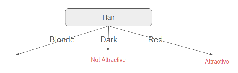
From these calculations, it follows that data must first be split with the Hair feature (which is the attribute with the maximum information gain).
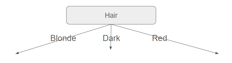
At this point, we can delve deeper because all the rows with Hair=Dark indicate not attractive people, while all the rows with Hair=Red indicate attractive people.
| Height | Hair | Eyes | Attractive ? |
|---|---|---|---|
| Tall | Red | Blue | Yes |
| Height | Hair | Eyes | Attractive ? |
|---|---|---|---|
| Tall | Dark | Brown | No |
| Tall | Dark | Blue | No |
| Small | Dark | Blue | No |
And then ?
We are now only concerned with people whose hair is blonde.
| Height | Hair | Eyes | Attractive ? |
|---|---|---|---|
| Small | Blonde | Brown | No |
| Tall | Blonde | Blue | Yes |
| Tall | Blonde | Brown | No |
| Small | Blonde | Blue | Yes |
We must proceed as before: computing the entropy of this new dataset and then find which feature (among Height and Eyes) has the maximal information.
$$H(S)=-\dfrac{2}{4}log_{2}\dfrac{2}{4} - \dfrac{2}{4}log_{2}\dfrac{2}{4}=1.000$$
$$H(S|Height)=\dfrac{|Height=Small|}{4}H(Height=Small)+\dfrac{|Height=Tall|}{4}H(Height=Tall)$$ $$H(S|Height)=\dfrac{2}{4}H(Height=Small)+\dfrac{2}{4}H(Height=Tall)$$
$$H(Height=Small)=-\dfrac{1}{2}log_{2}\dfrac{1}{2} - \dfrac{1}{2}log_{2}\dfrac{1}{2}=1.000$$ $$H(Height=Tall)=-\dfrac{1}{2}log_{2}\dfrac{1}{2} - \dfrac{1}{2}log_{2}\dfrac{1}{2}=1.000$$
We eventually have $H(S|Height)=1.000$ and therefore, $\boxed{IG(S, Height)=0.000}$.
$$H(S|Eyes)=\dfrac{|Eyes=Brown|}{4}H(Eyes=Brown)+\dfrac{|Eyes=Blue|}{4}H(Eyes=Blue)$$ $$H(S|Eyes)=\dfrac{2}{4}H(Eyes=Brown)+\dfrac{2}{4}H(Eyes=Blue)$$
$$H(Eyes=Brown)=-\dfrac{2}{2}log_{2}\dfrac{2}{2} - \dfrac{0}{2}log_{2}\dfrac{0}{2}=0.000$$ $$H(Eyes=Blue)=-\dfrac{2}{2}log_{2}\dfrac{2}{2} - \dfrac{0}{2}log_{2}\dfrac{0}{2}=0.000$$
We eventually have $H(S|Eyes)=0.000$ and therefore, $\boxed{IG(S, Eyes)=1.000}$.
From these calculations, it follows that data must now be split with the Eyes feature (which is the attribute with the maximum information gain). Moreover, it seems unnecessary to proceed further, as this feature already provides complete information about whether a person is attractive or not.
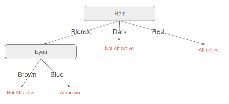
We can observe from this illustrative example that a person's height does not influence their attractiveness. This was not evident at all, even with this oversimplified dataset, and we end up with a very straightforward decision tree.
Test the decision tree
We can now use this tree to evaluate unforeseen samples. For example, is a small person with dark hair and brown eyes attractive ? We just have to follow the path to get the answer (it is no).
We can observe here the interconnection of data structures and machine learning. The response to a question involves traversing a path in a tree from the root to the leaf, and this traversal takes an average of $log(n)$ steps where $n$ is the number of nodes. Decision trees are therefore very efficient in providing quick answers, which explains their widespread use.
What's next ?
We haven't addressed continuous variables in this post. In fact, ID3 was initially designed for categorical data, and a new algorithm needs to be implemented for handling continuous variables. This will be the subject of the next article.