Truly understanding logistic regression - Part 3
In this post, we will outline the process of training the logistic regression algorithm.
In the previous post, we discussed that logistic regression involves stipulating that the outcome $C$ is a linear function of the features $x$ within the sigmoid's argument.
$$P(C|x)=\sigma(Wx+b)$$
Now, let's explore how to calculate the introduced parameters ($W$ and $b$). To illustrate these concepts, we will assume binary classification with classes $C_{1}$ and $C_{2}$, with the training dataset $D$ comprising $N$ records ($x_{1}$, ..., $x_{N}$), each encompassing $K$ features (observed variables).
Introducing the cost function
We will assume that the training data is independent and identically distributed, implying that each data point is statistically independent of the others and originates from the same probability distribution. Each observation is presumed to be drawn independently from this common underlying probability distribution. As a consequence, the joint probability is the product of the individual probabilities.
$$P(x_{1},...,x_{N})=P(x_{1})...P(x_{N})=\displaystyle\prod_{i=1}^NP(x_{i})$$
Let $i \in [1, N]$. If $x_{i}$ belongs to class $C_{1}$, then we have $P(x_{i})=P(C_{1}|x_{i})$. Otherwise, if $x_{i}$ belongs to class $C_{2}$, we have $P(x_{i})=P(C_{2}|x_{i})=1-P(C_{1}|x_{i})$. In all cases, we can express that $P(x_{i})=P(C_{1}|x_{i})^{t_{i}}(1-P(C_{1}|x_{i})^{1-t_{i}}$ where $t_{i}=1$ if $x_{i}$ belongs to class $C_{1}$ and $t_{i}=0$ if $x_{i}$ belongs to class $C_{2}$.
$$P(x_{1},...,x_{N})=\displaystyle\prod_{i=1}^NP(C_{1}|x_{i})^{t_{i}}(1-P(C_{1}|x_{i})^{1-t_{i}})$$
This quantity is referred to as the likelihood.
The objective now is to maximize the likelihood. To avoid issues with underflows, it is common to work with the logarithm of this quantity. Since the logarithm function is monotonically increasing, it does not affect the optimization. The cost function $E(W)$ is then defined as the negation, and the goal is to minimize this quantity.
$$E(W)=-\ln{\displaystyle\prod_{i=1}^NP(C_{1}|x_{i})^{t_{i}}(1-P(C_{1}|x_{i})^{1-t_{i}})}$$
$$\boxed{E(W)=-\displaystyle\sum_{i=1}^N(t_{i}\ln{P(C_{1}|x_{i})}+(1-t_{i})\ln(1-P(C_{1}|x_{i})))}$$
Minimizing the cost function
What we aim to do now is minimize the cost function. There are various methods for achieving this, such as different variants of gradient descent. In this post, we will choose to leverage the Newton-Raphson method by observing that minimizing $E$ involves nullifying its gradient.
$$\nabla E(w)=0$$
In this approach, we turn to the task of identifying the roots of a non-linear equation, and it is in this context that the Newton-Raphson method becomes instrumental.
Several optimization algorithms are possible, and the most commonly used ones are probably variants of gradient descent (such as stochastic gradient descent, conjugate gradient). Here, we present a method that leverages the Newton-Raphson algorithm.
For a comprehensive exploration of the topic, we recommend consulting the following textbook.
What is the Newton-Raphson method ?
While the Newton-Raphson method is not inherently challenging to grasp, complications can arise, and a rigorous examination of its convergence is far from trivial (see Wikipedia). For those proficient in French, further details can be found in Introduction à l'analyse numérique matricielle et à l'optimisation. Nevertheless, in practical scenarios, the sufficient conditions are often satisfied, and a perfect understanding of these intricacies may not be necessary.
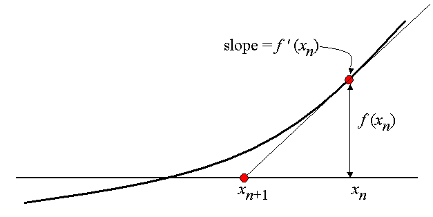
We will exemplify the method in one dimension and merely state the outcomes in multidimensions. At this juncture, we assume the presence of a differentiable function $f$ defined on an interval $I$. Our objective is to find a value $a$ such that $f(a)=0$, and we presume that we possess a preliminary approximation $x_{0}$ of $a$.
At this point, we can utilize the Taylor series expansion around $x_{0}$.
$$f(x)\approx f(x_{0})+(x-x_{0})f'(x_{0})$$
The method essentially refines the initial guess $x_{0}$ by taking into account both the function value and its slope $f'(x_{0})$ at that point. We define a new point $x_{1}$ by calculating the x-intercept of the tangent line at $x_{0}$.
$$f(x_{1})=0=f(x_{0})+(x_{1}-x_{0})f'(x_{0})$$
$$x_{1}=x_{0}-\dfrac{f(x_{0})}{f'(x_{0})}$$
As a result, a new point $x_{1}$ is obtained, representing a better approximation of $a$ than $x_{0}$. The iteration process continues until the difference between successive approximations is smaller than a predetermined tolerance level or until a maximum number of iterations is reached.
$$x_{k+1}=x_{k}-\dfrac{f(x_{k})}{f'(x_{k})}$$
When this method converges, the convergence is exceptionally rapid.
There exists a more useful version in multidimensional spaces, but it requires a deeper understanding of differential calculus and linear algebra. Once these intricacies are navigated, the results are very similar: we are now interested in solving the system of equations $F(x) = 0$ given a twice continuously differentiable function $F : \R^n \to \R^n$. In this scenario, the approach entails iterating the following sequence until the discrepancy between successive approximations becomes smaller than a predefined tolerance level or until a maximum number of iterations is attained.
$$x_{k+1} = x_{k}-JF(x_{k})^{-1}F(x_{k})$$
$JF$ is the Jacobian matrix. The Jacobian matrix is the matrix of all first-order partial derivatives of the vector-valued function $F$.
Applying the Newton-Raphson method
Recall that we aim to solve the equation $\nabla E(w)=0$ (with the preceding notations, $F=\nabla E(w)$).
Therefore, the Newton-Raphson method is expressed for the logistic regression as $w_{new}=w_{old}−(\nabla \nabla E)^{-1}\nabla E(w)$.
$$\boxed{w_{new}=w_{old}−H^{-1}\nabla E(w)}$$
$H$ is the Hessian matrix (i.e., "the derivative of the gradient"). It is important to note that we implicitly assume that the function to be minimized is twice continuously differentiable.
In practical application, this algorithm necessitates computing the inverse of a matrix, which can incur significant computational costs. Consequently, practitioners have turned to techniques that circumvent the need for explicitly calculating the Hessian matrix. Instead, the Hessian is updated iteratively by analyzing successive gradient vectors. This approach, known as quasi-Newton methods, can be viewed as a broader application of the secant method for multidimensional problems, aiming to find the root of the first derivative.
One of the most renowned and widely utilized quasi-Newton methods is the BFGS algorithm, which is implemented in the ML.NET framework.
And for logistic regression ?
The preceding calculations were fairly general and can be applied to any twice-differentiable function. Now, let us specifically apply them to logistic regression. The next step is to proceed with the computations by substituting the probabilities with the predefined sigmoid expression.
$$E(W)=-\displaystyle\sum_{i=1}^N(t_{i}\ln{P(C_{1}|x_{i})}+(1-t_{i})\ln(1-P(C_{1}|x_{i})))$$
But we imposed that $P(C_{1}|x_{i})=\sigma(Wx_{i})$ for all $i \in [1,N]$. After some intricate calculations and noticing that $\sigma '=\sigma (1-\sigma )$, we derive the following formula for the gradient and for the Hessian matrix.
$$\nabla E(W)=\displaystyle\sum_{i=1}^Nx_{i}(\sigma (Wx_{i})-t_{i})$$
$$H(W)=\nabla \nabla E(W)=\displaystyle\sum_{i=1}^N\sigma (Wx_{i})(\sigma (Wx_{i})-t_{i})x_{i}x_{i}^T$$
Using the property $0 \lt \sigma (Wx_{i}) \lt 1$ for all $i \in [1,N]$, which follows from the form of the logistic sigmoid function, we see that $u^THu \gt 0$ for an arbitrary vector $u$, and so the Hessian matrix $H$ is positive definite. It follows that the cost function is a convex function of $w$ and hence has a unique minimum.
Christopher Bishop (Pattern Recognition and Machine Learning)
The convergence is very rapid, enabling the parameters to be learned quickly through these iterations.
This algorithm is sometimes referred to as the iterative reweighted least squares (IRLS).
We have presented the framework for binary classes here. All these findings can be extended to $K$ classes, where the link function is no longer a sigmoid but the softmax function. The Newton-Raphson method can still be utilized to train the parameters in this generalized context.
In modern machine learning libraries, this method is implemented using the widely-used L-BFGS algorithm. This variant should be properly referred to as a quasi-Newton algorithm, as the Hessian matrix is not explicitly computed but updated by analyzing successive gradient vectors instead.
How to predict an unforeseen input ?
Once the logistic regression has been trained using the Newton-Raphson method, it becomes possible to make predictions. From an input $x$, we can calculate the probability for each class $C_{k}$ using the formula derived earlier ($P(C_{k}|x)=\sigma (W^Tx)$) and select the category with the highest probability as the predicted outcome.
Certainly, enough theory for now. It's time to put this knowledge into practice. Let's apply these formulas using the ML.NET framework.